by R. Grothmann
The simple Lagrange method relies on the fact that a minimum of f(v) under the condition g(v)=0 has the property that the
![]()
The only condition is that the grad g(v) is not zero, and both functions are continuously differentiable.
Euler loads two functions getlagrange() and solvelagrange() into Maxima. But we want to try the solution step by step first.
The easiest way to set up the necessary equations is the Lagrange function f+cg. We demonstrate that in an example. We want to minimize
![]()
subject to x+y=1.
>f &= x^(4/5)*y^(1/5)
                               4/5  1/5
                              x    y
>g &= x+y-1
y + x - 1
>L &= f+c*g
                                       4/5  1/5
                      c (y + x - 1) + x    y
Maxima can solve this.
>&solve(gradient(L,[x,y,c]),[x,y,c]); sol &= %[1]
                                            8/5
                           4      1        2
                      [x = -, y = -, c = - ----]
                           5      5         5
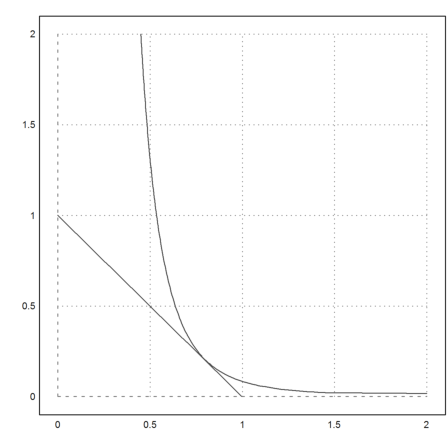
We can plot this optimal solution in Euler. The colored line is the condition g=0.
>plot2d(f,level=f(4/5,1/5),a=0,b=2,c=0,d=2,n=100); ...
 plot2d(g,level=0,add=1,color=5,n=100):

The optimal value is the following.
>&f with sol
                                  4/5
                                 4
                                 ----
                                  5
From the image it is clear, that the optimum is a maximum. One way to prove this is a special Hessian matrix.
>H &= matrix([0,diff(g,x),diff(g,y)], ...
   [diff(g,x),diff(L,x,2),diff(diff(L,x),y)], ...
   [diff(g,y),diff(diff(L,x),y),diff(L,y,2)])
                  [ 0       1             1       ]
                  [                               ]
                  [          1/5                  ]
                  [       4 y             4       ]
                  [ 1   - -------    ------------ ]
                  [           6/5        1/5  4/5 ]
                  [       25 x       25 x    y    ]
                  [                               ]
                  [                        4/5    ]
                  [         4           4 x       ]
                  [ 1  ------------   - -------   ]
                  [        1/5  4/5         9/5   ]
                  [    25 x    y        25 y      ]
If the determinant of this matrix is positive, we have a local maximum.
>&H with sol, &:determinant(%)
                       [ 0     1        1    ]
                       [                     ]
                       [                4/5  ]
                       [        1      4     ]
                       [ 1  - ------   ----  ]
                       [         1/5    5    ]
                       [      5 4            ]
                       [                     ]
                       [       4/5       9/5 ]
                       [      4         4    ]
                       [ 1    ----    - ---- ]
                       [       5         5   ]

3.78929141628
Note that is easier in this example to solve the codition g=0 for y, and to insert that into the f.
>&solve(g,y), &f with %, solx &= solve(diff(%,x)=0,x)
                             [y = 1 - x]


                                  1/5  4/5
                           (1 - x)    x


                                    4
                               [x = -]
                                    5
It is also easy to compute the second derivative for this function. So we can prove a local maximum.
>&solve(g,y); &f with %; &diff(%,x,2) with solx | float
- 3.789291416275997
Indeed the second derivative is less than 0 everywhere for 0<x<1. So it is an absolute maximum. We know that already, since it the only zero of the derivative in that interval, and a local maximum.
>&solve(g,y); &f with %; &diff(%,x,2)|factor
                                  4
                      --------------------------
                                4/5          6/5
                      25 (1 - x)    (x - 1) x
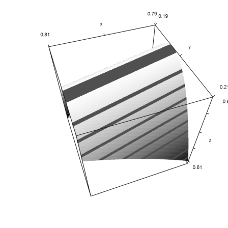
The Lagrange function has a maximum in the point. But it is not possible to see this with the Hessian matrix.
>Lag &= f+c*g with c=(c with sol), &eigenvalues(hessian(Lag,[x,y]) with sol)
                                  8/5
                      4/5  1/5   2    (y + x - 1)
                     x    y    - ----------------
                                        5


                             17
                       [[- ------, 0], [1, 1]]
                              1/5
                           5 4
A detailed plot shows the situation.
>plot3d("Lag(x,y)",r=0.01,cx=0.8,cy=0.2, ...
   angle=160°,height=50°,>contour):

We can try to solve this system numerically. To setup the equations, we use calls to Maxima at compile time.
It turns out that we have to be careful with negative x and y. The algorithm gets into these regions easily.
>function lg([x,y,c]) ...
   x=abs(x); y=abs(y);
   return [&:"diff(@f+c*@g,x)", ..
     &:"diff(@f+c*@g,y)", ..
     &:"diff(@f+c*@g,c)"]
 endfunction
Now start the Broyden algorithm.
>broyden("lg",[1,1,-1])
[0.8, 0.2, -0.606287]
The Nelder Mead method works too.
>function h(v) := norm(lg(v))
>neldermin("h",[1,1,0])
[0.8, 0.2, -0.606287]
Euler loads some additional Maxima commands on startup. One of them is the solvelagrange method.
>&solvelagrange(f,g,[x,y])
                               8/5
                              2         1      4
                   [[lambda = ----, y = -, x = -]]
                               5        5      5
Let us try a higher dimensional problem. Find the extremal values of x*y^2*z^3 for x+y+z=1.
>sol &= solvelagrange(x*y^2*z^3,x+y+z-1,[x,y,z])
        [[x = %r1, lambda = 0, z = 0, y = 1 - %r1],
[x = %r2, lambda = 0, z = 1 - %r2, y = 0],
     1           1       1      1
[x = -, lambda = --, z = -, y = -],
     6           72      2      3
     1                         2
[x = -, lambda = 0, z = 0, y = -], [x = 0, lambda = 0, z = 1, y = 0]]
     3                         3
The interesting solution is the third one, of course. Since f approaches 0, whenever x, y, or z approach 0, we know that this must be a global maximum.
>&[x,y,z] with sol[3]
                               1  1  1
                              [-, -, -]
                               6  3  2
We can also just print the Lagrange equations.
>&getlagrange(x*y^2*z^3,x+y+z-1,[x,y,z])
          2  3                  3                2  2
        [y  z  = lambda, 2 x y z  = lambda, 3 x y  z  = lambda,
                                                    z + y + x - 1 = 0]
We show in an example, how to solve a Lagrange-Problem with the Newton algorithm.
>function g(x,y) &= x^2*y+y^2*x+x^4-1
                            2    2      4
                         x y  + x  y + x  - 1
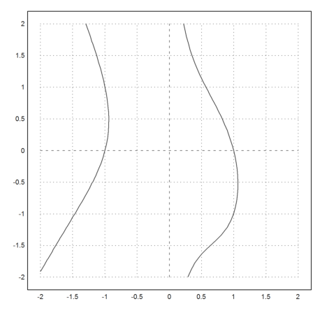
Here is a plot of the set g(x,y)=0.
>plot2d("g",level=0,r=2):

We seek the point of minimal distance to (1,1).
>function f(x,y) &= (1-x)^2+(1-y)^2
                                2          2
                         (1 - y)  + (1 - x)
The Lagrange function looks like this.
>L &= f(x,y)+lambda*g(x,y)
             2    2      4                      2          2
         (x y  + x  y + x  - 1) lambda + (1 - y)  + (1 - x)
We wish to find a zero of L'(x,y,lambda)=0.
>function dL([x,y,lambda]) &= grad(L)
           2              3
        [(y  + 2 x y + 4 x ) lambda - 2 (1 - x),
                          2                         2    2      4
                (2 x y + x ) lambda - 2 (1 - y), x y  + x  y + x  - 1]
For the Newton algorithm, we use Maxima to compute the Jacobian of dL.
>function DdL([x,y,lambda]) &= jacobian(dL(x,y,lambda),[x,y,lambda])
   [            2                                   2              3 ]
   [ (2 y + 12 x ) lambda + 2  (2 y + 2 x) lambda  y  + 2 x y + 4 x  ]
   [                                                                 ]
   [                                                           2     ]
   [    (2 y + 2 x) lambda       2 x lambda + 2       2 x y + x      ]
   [                                                                 ]
   [     2              3                   2                        ]
   [    y  + 2 x y + 4 x           2 x y + x               0         ]
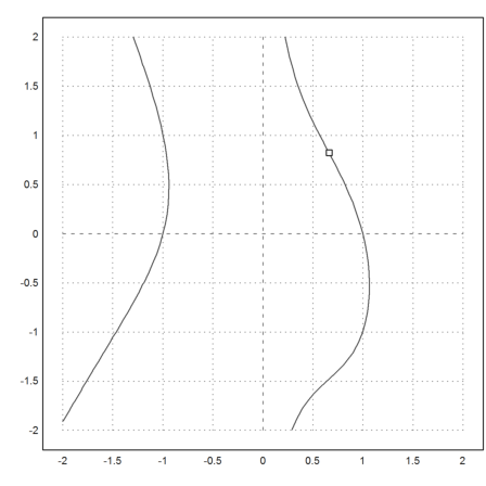
Now we can run the algorithm, and add the solution to the plot.
>newton2("dL","DdL",[1,1,0]), plot2d(%[1],%[2],points=true,add=true):
[0.661468, 0.823282, 0.231505]

In fact, this can be numerically solved by Maxima. Many solutions are imaginary, but there is the following solution among them.
>&solve(dL(x,y,lambda))[6]
        [lambda = 0.23150453851715, y = 0.82328207592504,
                                                 x = 0.66146848602989]
The interval Newton method works too. The inclusions are guaranteed.
>{xsol,valid}=inewton2("dL","DdL",[1,1,0]); xsol,
[ ~0.6614684927715179,0.6614684927715191~,
~0.8232820646967926,0.8232820646967943~,
~0.2315045435202875,0.2315045435202889~ ]
>valid,
1